Bonds: Probit Models Predict Probability Of Recession

There was much ado over Greenspan's recent comments that there is a 33% chance the U.S. economy will enter into a recession later this year. The Fed seemed to be caught off guard by these comments, and Bernanke testified before Congress that The Fed was still concerned about inflation and the economy is in good shape. Why would Greenspan make such remarks?

We believe it is highly likely that Greenspan's forecast is based on probit models designed by The Fed. For those of you who aren't familiar with a probit model, we will look at the following definitions of probit. Wikipedia's definition is: "In statistics, a probit model is a popular specification of a generalized linear model, using the probit link function. Probit models were introduced by Chester Ittner Bliss. Because the response is a series of binomial results, the likelihood is often assumed to follow the binomial distribution." About Economics defines probit as: "An econometric model in which the dependent variable yi can be only one or zero, and the continuous independent variable xi are estimated in:

Pr(yi=1)=F(xi'b)

Here b is a parameter to be estimated, and F is the normal cdf. The logit model is the same but with a different cdf for F."

For those who still don't know what a probit model is, let's just say it is an econometric forecasting model. Probit models have been used by The Fed to forecast recessions. These models are based on the slope of the yield curve and have been very reliable in forecasting periods of economic weakness. When the 90 day T-Bill yields more than the 10 Year treasury bond, the model views this as a negative development for the economy. The chart below shows the history of the 10 Yr vs. the 90 Day T-Bill for the last 20 years.


Jonathan Wright from the Federal Reserve Board's Division of Monetary Affairs developed a probit model that measures the spread between the 3 month T-Bill yield and the 10 Year Treasury yield. It also looks at the general level of Fed Funds. He has written a working paper entitled "The Yield Curve and Predicting Recessions" which compares 4 different versions of the model. He concludes that measuring the spread between the 3 month T-Bill and the 10 Year Treasury as well as including the level of Fed Funds is the best of the 4 approaches for predicting recessions. The results of the model are shown below. The number at the right is the probability of a recession and the red areas show periods of economic weakness. As you can see, this model has had a very close correlation when predicting periods of economic weakness in the past without giving false signals.


Griffin Kubik, a securities firm in Chicago, replicated this model. The model is currently saying there is a better than 50% chance of a recession in the next 4 Quarters. We have seen other models projecting as high as a 95% chance of recession. Some of these other models are based on the spread between the 1 Year T-Bill and the 10 Year, without factoring in the general level of interest rates. Wright enhanced these earlier models by including Fed Funds as a proxy for interest rates. It seems likely that Greenspan is using some variation of one of these types of probit models. Perhaps he has enhanced Wright's model with some other variable. Although each of these models project different probabilities for a recession, they all agree that the longer The Fed keeps the yield curve inverted, the greater the probability our economy will enter a recession by the end of the year. The chart below shows the current estimation of the probability of a recession using Wright's model. Remember the probability was only at 20% when the chart above was created.

Taxes: The Battle Over AMT

It is estimated that the Alternative Minimum Tax, if left unchanged, will raise about $50 billion this year for the Federal Government. This is a tax implemented by Congress several years ago to make sure wealthy individuals pay their "fair share" of taxes. This tax was not indexed to inflation and is now affecting many members of the not-so-wealthy middle class. There is considerable ongoing debate about what to do about the AMT in Congress, because it is not fair to leave it as it is. The Republicans would like to either repeal the tax or mend it for another year. The Democrats would like to change the tax so that more of the tax is paid by the wealthy and eliminate the Republican tax cuts from 2001 and 2003,which are set to expire in 2010, as a way to pay for the AMT fix.

Congress has consistently over-estimated it's ability to implement a "fair" tax code, and under-estimated the impact on the American people and our economy of constantly changing the code. The Alternative Minimum Tax is a good example of why it is time for a change in how Congress views taxes. We believe the Government has proven it's inability to create a fair tax system. Instead, they should simplify the code and beef up the enforcement division of the IRS. A simpler tax code would help to narrow the tax gap and the AMT could be eliminated without having to fret over the $50 billion in lost revenues it generates this year.

The Wall Street Journal on March 21,2007 had an article discussing the current Tax Gap because of under-reporting of taxes due. This amount is estimated to be $345 billion. The table/chart below shows the composition of the tax gap and the decline in the number of IRS enforcement agents over the last 10 years.



We believe much of this under-reported income is caused by the complexity of the existing tax code. The first step for Congress should be to simplify the code. The current system of graduated brackets, deductions, and exceptions creates incentives for taxpayers to find ways around paying taxes. The more complicated we make our tax system, the more money falls through the cracks. For example, a flat tax with no deductions would be simple and easy to implement and enforce. Some may say that a flat tax would be unfair. Our answer to that is: "How fair is it that we are paying taxes and there are $345 billion of taxes owed that others aren't paying?"

Bonds: How Strong Is The Economy?

The Index of Leading Economic Indicators is showing potential economic weakness in the months ahead. The chart below shows the LEI for the last 15 years. The LEI peaked out in January 2006 at 139.1. The levels for February, which were just released, show a reading of 137.3. This index is a good indicator of economic strength over the next 4-6 months. The weakness in this indicator would suggest slower growth or weakness for the balance of 2007.

The LEI is composed of 10 different components. The different components are listed below with both their weighting in the index and their contribution to the last reading of LEI. The Conference Board releases this data about 3 weeks after the end of the previous month.

The largest contributors to the LEI are the Money Supply and the Factory Workweek. These 2 components account for about 60% of the value of the LEI. Recently, there has been much talk in the press about the housing market and whether the weakness in housing will drag down the rest of the economy. This sector of the economy is measured by Building Permits which accounts for only 2.7% of the LEI. However, most of the focus of economists and the press has been on housing. Now, their attention is moving to high defaults in sub-prime mortgages, and possible tightening of credit conditions for new home buyers.

Let's look at the LEI and some of the other components of the index. Last month, 5 of the 10 measures showed weakness in the economy. These measures were: the yield curve, vendor performance, initial jobless claims, consumer expectations, and building permits.

There is value in following the LEI and all of these components. The weakness in the index is not coming from only 1 sector of the economy (housing), but is shown in several of the individual measures of future economic growth. There are several economists calling for the economy to pick up later in the year. (These economists are obviously not paying attention to the LEI). We feel this is unlikely, and expect the economy to continue to slow. This should provide a favorable backdrop for bonds.

All data shown above is from the Conference Board which releases the Index of Leading Economic Indicators.

Taxes: Tax Freedom Day

This is the time of year to be thinking about taxes. We believe that each investor has a unique tax situation, and we are concerned about their marginal tax rates in the selection process of individual securities for their fixed income portfolios. We believe the last elections were a watershed event for tax rates, and that marginal tax rates are likely to rise in the future. This will probably make tax-free securities more attractive compared to taxable securities for some investors in the future.

The Tax Foundation publishes some interesting data about taxes and their impact on our daily lives. As a way to show how much of our income we pay in taxes, they created Tax Freedom Day. If we assume that we pay our taxes before we can use the rest of our earnings, this would be the day that we are "free" of paying taxes and the rest of our earnings go to us. The later in the year we reach Tax Freedom Day, the more time we are working for the government and the less time we are working for ourselves. This is a valuable way of measuring the bite that taxes are taking from our paychecks, and allows for comparisons over time. The chart below shows Tax Freedom Day for the last 27 years. The axis on the left shows the number of days it takes to get to Tax Freedom Day and the graph shows the results over time. We reached a high of about 123 days in 2000 and now are working about 116 days for the government.


How much do you pay in Federal taxes and how much do you pay in State & Local taxes? The chart below begins in 1900 and shows the number of days over time you work for each of these.

If you are wondering how many days you work to pay for your taxes compared to how many days you work to pay for housing, the chart below gives you the answer. We work 77 days to pay Federal taxes, 39 days to pay State & Local taxes, and 62 days to pay for housing and household operation. Federal taxes is the largest category.

You may also be wondering how the different taxes break down by type of tax. Below is a chart that shows the types of taxes. For example, out of the 77 days you work to pay for Federal taxes, 30 days go to pay for social programs such as Social Security and Medicare.

The amount of time you spend working for the government depends upon where you live. The chart below shows you will be working harder for the government if you live in New York than if you live in Montana. The states in dark blue mean that Tax Freedom Day occurs later in the year than the light blue and white states. We would encourage you to visit the website for the Tax Foundation for further information. We have provided a link to their website on our blog for your convenience.

Muni Bonds: Why Buy Premium Coupons?

Premium Coupon Bonds Are Less Risky

Bonds purchased at par (a dollar price of 100) are considerably more risky than premium coupon bonds for three different reasons. First, the duration is greater for a par bond. Second, the reinvestment of interest earned has less of an impact on total return. Finally, in a rising rate environment, par bonds become subject to the Market Discount Rule more quickly.

Most investors purchase bonds as a way to dampen the volatility of their whole portfolio and to create a stream of income. Since the bond portfolio is used to reduce overall risk, it makes sense to reduce the risk taken in this conservative part of the portfolio whenever possible. The purchase of premium coupon bonds is a natural way for the fixed-income portfolio manager to reduce the risk for his investors.

An Example of Bond Cash Flows

There was a Michigan Trunk muni bond issue that came the week of August 16, 2004 consisting of par bonds and premium bonds in the same maturities. The original pricing was the same for both coupon structures (3.77% yield). The par bonds were 3.75% due to mature on 9/1/14 and the premium bonds are 5.0% maturing on the same date. The following is a comparison of these two different coupon structures. Assume that about the same amount of money is invested in each bond. Both structures will provide about the same amount of total income or cash flows, if held to maturity.


The par bonds will consist of a greater par value of bonds ($1,000,000 vs. $906,000), but will have lower coupon payments than the premium bond ($375,000 vs. $453,000). The coupon payments are assumed to be reinvested at the purchase yield of 3.77%. The par bond will earn less reinvestment income than the premium bond ($73,395 vs. $91,078). Note: This illustration allows us to purchase a $906,000 block of bonds. Munis come in $5,000 denominations, but this example more accurately shows how the cash flows work.

Duration

The table shows the duration for the par bond is 8.248 at the time of issue. The duration for the 5.0% coupon is 7.927. Since the 5.0% coupon has the lower duration, it is the less risky of the two structures. Duration is a measure of market or interest rate risk. The greater the duration, the more market risk the investor is taking. Duration is similar to beta for stocks, where beta is the amount of risk the investor is taking compared to the risk of the market. One way to think of duration is as a measure of how much the price of an individual bond would change with a 1% change in interest rates. A bond with a duration of 4.0 would have a price change of about 4.0%. In our example, the par bond would change .321% more than the premium bond because of market risk (8.248-7.927).


Reinvestment of Interest Earned

The premium bond receives more cash flows from coupon payments ($453,000 vs. $375,000). The reinvestment of these cash flows creates additional interest earned for the investor. Since the cash flows received from coupon payments are greater for the premium bond, the amount of interest earned from reinvestment is also greater. In this example, we assume the reinvestment rate rises 1.0% to 4.77. This creates $4,479 in additional income for the investor in the premium bonds. This is a favorable characteristic in a rising rate environment. The investor is receiving his money back more quickly which allows him to reinvest it at higher rates (if rates rise).

Market Discount Rule

Avoiding the Market Discount Rule is the most important reason to invest in premium coupon bonds. The Market Discount Rule assigns a price (yield) for each security when it is purchased. If yields rise above that pre-assigned yield, the market would penalize the investor's security if the investor needed to sell the bond because the difference between the purchase price for the new investor and the price he receives at maturity would be taxed as ordinary income. This has a very negative impact on an individual security’s value. Most investors purchase muni bonds because they want tax-free income. Discount bonds cheaper than the market cut-off price will need to appeal to an investor willing to earn taxable ordinary income which is (in the case of the high net worth individual) most likely taxed at the maximum tax rate. Our example shows that the par bond has a market cut-off or QTAX of 4.05. If market yields were to rise to 4.77% for this maturity, the par bond would likely have to trade at a yield of 5.34% in order to entice investors to purchase the bonds. This extra yield is necessary because the difference between the purchase price of $88.751 and the price received at maturity (par or 100) is taxed at the taxpayers ordinary income tax-rate.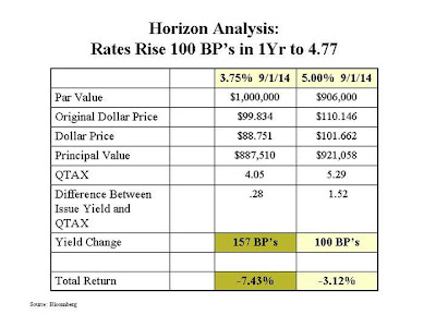

The premium bond would avoid this Market Discount Rule problem and would decline in value by (3.12%) vs. the decline in value of the par bond by (7.43%).

As you can see, the Market Discount Rule can have a very significant impact on total returns in a rising rate environment.

Who Buys Par Bonds?

The primary purchasers of par bonds are bank trust departments and individuals. Bank trust departments buy par bonds because of the nature of the trust relationship. In every trust, there is an income beneficiary and a remainder man. It is the trustee’s responsibility to make sure both parties are treated fairly. Tradition has argued that the best way to ensure fairness is to purchase par bonds. Remember that a bond consists of a series of cash flows. If a premium coupon bond is purchased and all of the income received is paid out, the remainder is less than what the remainder man would ordinarily be entitled to (part of the income is really amortized premium or principal). One has to question this logic, however. Is the remainder man of the trust being treated fairly if the market value of his holdings declines because of the market discount rule? One could argue that the trust department could still buy premium bonds and only pay out that portion to which the income beneficiary is entitled. This approach requires more work for the trust department, but is a lower risk strategy for the trust as a whole.

Retail investors or individuals typically purchase par bonds because they don’t understand how bonds work and they may not have the tools necessary to analyze bond cash flows properly. Bond risks are difficult to measure and not readily understood by many retail investors.

Conclusion

Risk management is a major component of managing a municipal bond portfolio. This example shows that premium coupon bonds are less risky than par bonds because they have less market risk, reinvestment risk is lower in a rising rate environment, and the risk associated with bonds becoming subject to the Market Discount Rule is greater for par bonds.

These are the reasons that most institutions and other savvy investors have been attracted to investing in premium coupon municipal bonds.

Bonds: Tax-Free, Taxable, Or Both?

The Problem
Perhaps one of the most confusing decisions facing an investment advisor today is whether some clients with taxable accounts should purchase taxable or tax exempt bonds for their high quality bond portfolios. This decision is straightforward for clients that earn large amounts of taxable income (over $326,450) which puts them into the maximum tax bracket of 35%. Municipal bonds are clearly the most appropriate investment for them. However, this decision is much more difficult when the client has invest able funds of $1-$3 million and very little (if any) taxable income coming from other sources. In these cases, the investment chosen “drives” the amount of taxable income that the client earns as well as their marginal tax bracket. For example, assume the client has an investment portfolio of $3.5 million and taxable income of $100,000. The portion the advisor allocates to the high quality bond portfolio is $800,000. Most advisors struggle with the appropriate mix of bonds for these clients. “Should I buy taxable bonds, tax exempt bonds, or perhaps a mix of both?” What is the proper way to make this investment decision?

Interest rates are constantly changing and so is the relationship between taxable and tax exempt securities along the yield curve. The changes in both interest rates and the inter-market relationships are important factors in the decision making process. The combination of changing rate levels as well as changing income levels makes this decision appear to be challenging.

Marginal Tax Rates
Tax-managing bond portfolios begins with a careful examination of the client’s marginal tax rate. This rate will determine the suitability of different fixed income securities for each client. This rate is dependent on the type of filing of the taxpayer and the level of income the client earns after all deductions are subtracted.

Filing Status
A single person has a higher marginal tax rate for the same level of income than a married person filing a joint return.

Income
We are referring to taxable income after all allowable deductions have been taken. This is the number from line 43 of the 1040 return. This income number can be used to determine the client’s marginal tax rate. Securities available in the tax-exempt and taxable markets can then be compared on an after-tax basis. These after-tax rates are then compared by maturity to determine what works best for each client. These rates and relationships are changing on a daily basis. Frequently, the portfolio is optimized by using a combination of longer maturity munis and shorter maturity agencies.

More emphasis needs to be placed on determining each client’s marginal tax rate. This may be difficult because of the many variables involved which causes this rate to be a “moving target.” Superior bond portfolio performance depends on improving this process.

Ratio of Munis to Agencies
The muni yield curve can be compared to the taxable yield curve to determine the percentage that each of the maturities trade compared to taxables. Munis traditionally trade at lower ratios in the shorter maturities and higher ratios in the longer maturities. The chart below shows the historical ratio of a 10 year muni compared to a 10 year U.S. Treasury bond. The average for the last 3 years is 86%. Recently, this ratio has fallen to 82.4%. This has an impact on after-tax yields and means that an investor needs to be in a higher tax bracket (86%-82.4%=3.6%) for munis to be attractive. This change is about equal to the amount of state tax a married person filing jointly would pay in the state of Arizona.

One way of looking at the current value of a muni compared to a taxable security is to take the ratio (munis/taxable's) and subtract it from 1. We can do this for all maturities along the curve and we get a chart like the one titled Muni/Agency Ratio which shows tax efficiency below. If we compare this graph to the client’s marginal tax rate (the blue line), we can see that munis will be attractive to the investor whenever this ratio is lower than the marginal tax rate. Munis are only attractive to this investor when he begins to look at maturities in the 5 year part of the curve. Munis would be attractive to all investors in the 35% bracket or higher. The advantage of this approach is that the tax-free/taxable ratio is constantly changing. We can monitor the ratios up and down the yield curve and compare them to the client’s marginal tax rate to determine which fixed income security is best suited for his/her needs.
Conclusion

Each individual investor has a unique tax situation. Returns may be optimized when more attention is paid to the marginal tax rate of each client. This requires familiarity with the client's tax return, and an understanding of the client's tax situation.

So You Think You Want To Be A Credit Analyst: Unfunded Pension Liabilities

Recently, S&P released a report entitled "Improved U.S. State Pension Funding Levels Could Be On The Horizon." This report is based on 2005 year-end data, which is the most recent data available for all states. S&P made the case that most state pension funds use 5 Yr smoothed returns, and the returns from 2001-2002 have been acting as a drag on the actuarial value of fund assets. If the equity market behaves itself, the 5 Yr smoothed value of these assets will increase as the returns from 2001-2002 fall off the 5 Yr averages. This increase in asset values will increase the funding of these state pension systems, which will help alleviate the current levels of underfunding. We are in agreement with this conclusion; however, there are some states that are grossly underfunded. Let's take a look at these state retirement plans and see how municipal credits are analyzed.

The chart below shows the 10 states with the largest Unfunded Actuarial Accrued Liabilities (UAAL). California, at $47 billion, has the largest unfunded liability, Illinois is next with $31 billion, and Ohio is right behind with $30 billion. The rest of the top 10 are all under $15 billion.

While it is interesting to know the magnitude of the funding gap, it is beneficial to look at the percentage that is funded to determine the progress the state has made in providing money for these obligations. The chart below is based on data from the same S&P report as above. This chart ranks states by the percentage of the funding. West Virginia has the lowest value at only 47% funded, next is Oklahoma at 57%, and Connecticut at 58%.

We now have charts that show the magnitude of the shortfall and the progress each state has made in achieving their goal of funding these pension obligations. It is also important to see how well these states can afford to meet these pension obligations. The amount of debt each state has outstanding can be calculated. If we divide this number by the population of the state, we arrive at a number for Debt Per Capita. Let's take the amount of the unfunded liability and divide it by the population to arrive at the Per Capita Unfunded Liability. When these 2 numbers are combined, we have a measure that is a better representation of the total obligation of the state. There are also Per Capita income numbers available for each state. These numbers show the earning power of the average person in the state. The combined Debt Per Capita numbers divided by the Per Capita income number gives us the percent of debt to income for each person. This number helps to show how significant the debt burden is for taxpayers in any given state. The chart below shows these numbers for the 10 states with the highest combined debt burden compared to their earning power. All 10 states have 10% or more ratios, with Alaska over 20%. This may be easier to understand if we use some actual numbers. Let's use Alaska as an example. The Debt Per Capita (PC) is $2,000 and the Unfunded Pension Liability is $6,212 PC. This is a total of $8,212 PC divided by the PC Income of $35,612 to give us a debt ratio of 23%. This is a big number and should cause concern in some investors. This measure gives us a better idea of Alaska's financial health than the $2,000 Debt Per Capita number.

These numbers do not include OPEB liabilities. OPEB is Other Post Employment Benefits and is primarily the actuarial accrued liability for health care costs. States will be coming out with these numbers over the next 3 years as required by GASB 45. This is another huge liability that municipalities have incurred. It should be important to each investor to look at not only traditional numbers such as Debt Per Capita, but also to include unfunded pension liabilites and OPEB obligations in their analysis to determine the creditworthiness of each security. So, do you still think you want to be a credit analyst?